Image Compression using K-Means Algorithm
So far, all the post discussed here belong to the category of supervised learning. In this particular post, we will bring up unsupervised learning! Contrary to supervised learning, supervised learning uses an unlabeled training set rather than a labeled one, where we do not have the vector of expected results, we only have a dataset of features where we can find its structure.
One fine example of unsupervised learning is clustering. When explained in a non-technical way, it is same to the English saying, birds of a feather flock together! Clustering is widely applied in solving many modern day problems, ranging from marketing, social media, medical, astronomy and many more…Today we will discuss one of the most popular and often used algorithm - K-means Algorithm - for automatically grouping data into coherent subsets ( refer to the number of clusters), where members of each cluster will share similar patterns.
Imagine if we decided to use = 2, then the pseudo-code of K-means Algorithm is as follows:
Randomly initialize K cluster centroids mu(1), mu(2), ..., mu(K)
Repeat:
   for i = 1 to m:
      c(i):= index (from 1 to K) of cluster centroid closest to x(i)
   for k = 1 to K:
      mu(k):= average (mean) of points assigned to cluster k
The first for-loop is the ‘Cluster Assignment’ step, where we make a vector where represents the centroid assigned to example .
The second for-loop is the ‘move centroid’ step where we move each centroid to the average of its group.
There are a few conventions to measure the distances, this example will use the Euclidean distance to compute distance, where
Going back to the above-mentioned pseudo-code, when translated to simple words, they would mean:
1. Randomly initialize two points in the dataset called the cluster centroids.
randidx = randperm(size(X,1));

centroids = X(randidx(1:K), :);
2. Cluster assignment: assign all examples into one of two groups based on which cluster centroid the example is closest to
for i = 1:length(idx)
  % we set the distance to a vey big number
  % for each iteration, the distance will gradually reduced
  % ie closer distance will be chosen
  min_distance = realmax();
  for j = 1:K
    % we use the norm() function to calculate the euclidian distance
    dist = norm(X(i,:)- centroids(j,:));
    if(dist < min_distance)
      min_distance = dist;
      % then we assign the cluster that data point belongs to
      idx(i) = j;
    end
   end
end
3. Move centroid: compute the averages for all the points inside each of the two cluster centroid groups, then move the cluster centroid points to those averages.
for i = 1:K
  % determine indices which belong to the first, second....nth cluster
  % then find the average for each cluster
  % we use the find() function to help us determine those indices
  index_i = find(idx == i)
  centroids(i,:) = sum(X(index_i,:)) / length(index_i);
4. Re-run Step 2 and Step 3 until the averages do not change any more.
Before we discuss about our optimization objective, let us understand some of the variables used:
- = index of cluster(1,2,…) to which example is currently assigned
- = cluster centroid
- = cluster centroid of cluster to which example has been assigned.
Our the cost function we are trying to minimize is as follows
where we will be finding all the values in the sets , representing all our clusters, and , representing all our centroids, that will minimize the average of the distances of every example to its corresponding assigned cluster centroid.
For the sake of illustration, we will use a dummy data to demonstrate the idea of K-means Algorithm. The following table will show how the centroids are shifted.
| Iterations | |
|---|---|
As observed from the above illustrations, notice the initial positions of the centroids changes from iteration to iteration. These centroids will slowly converge to a point where the they cannot converge any where further.
Image Compression with K-means Algorithm
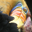
Now that we have understand the fundamental theory behind K-means Algorithm, we will apply this concept to compress a cute bird image, like in Figure 1, where Figure 1 is an image of a thousand colors.
 Figure 1: Our original 128x128 image.
In a typical RGB encoding, an image is represented using 24 bits, where each pixel is represented as three 8-bit unsigned integers (ranging from 0 to 255) the Red, Green and Blue intensity values, hence the name RGB.
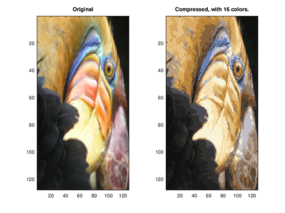
Here, we will be using 16 () colors to represent our cute bird, and for each pixel in our image we now need to only store the index of the color at that location, i.e. where only 4 bits are necessary to represent 16 possibilities ().
With the help of image packages in Octave/Matlab, our images can be easily represented with number.
% Octave/Matlab implementation
Image = imread('original.png');
This will create a 3D matrix Image whose first two indices identify a pixel position and whose last index represents either Red, Green or Blue. For instance, Image(30,40,3) gives the blue intensity of the pixel at row30 and column40.
Once we implement our K-Means Algorithm with , we will be able to compress our cute bird into as follows
 Figure 2: Our original image vs. Compressed image using 16 colors.
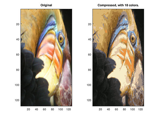
We can easily change the number of to study the effects it brings to image compression, Figure 3 and Figure 4 shows the result of the compressed image using and respectively.
Figure 3: Our original image vs. Compressed image using 14 colors.
 Figure 4: Our original image vs. Compressed image using 18 colors.
Conclusion
This covers pretty much the fundamentals of K-Means Algorithm. But before that, it is also interesting to bring up the issue on choosing the number clusters. There has been an endless debate on whether what number of clusters will perform best, however, this is a very subjective question and can be quite arbitrary and ambiguous. The Elbow method is widely used as the rule of thumb to determine the number of clusters, where we plot the cost function and the number of clusters . should reduce as we increase the number of , and then flatten out. Finally, we choose at the point where the cost function starts to flatten out. However, in real world problems, the chance of getting a clear elbow is often very slim.
To really determine the number of , one should really understand what kind of problem that is being solve instead of relying on methods to determine the number of , because for the same number of , when applied to different problem, it could provide an entirely different landscape to the problem.
To conclude, the following table shows the strengths and weaknesses of this unsupervised learning method
| Strengths | Weaknesses |
|---|---|
| Uses simple principles that can be explained in non-statistical terms | Not as sophisticated as more modern clustering algorithms |
| Highly flexible, and can be adapted with simple adjustments to address nearly all of its shortcomings | Because it uses an element of random chance, it is not guaranteed to find the optimal set of clusters |
| Performs well enough under many real-world use cases | Requires a reasonable guess as to how many clusters naturally exist in the data |
| Not ideal for non-spherical clusters or clusters of widely varying density |