Email Spam Classifier with Support Vector Machine (SVM)
Support Vector Machine (SVM) is another kind of supervised machine learning algorithm and can be imagined as a surface that produces a boundary between points of data plotted in multi-dimensional that represent examples and their features values. The ultimate goal of a SVM is to produce a flat boundary called a hyperplane, which separates the space to create fairly similar partitions on either side.
Our SVM has a cost function of
where and is used as a regularization parameter. Therefore, when we want to regularize more i.e. reduce over-fitting, we decrease , and when we want to regularize less i.e. reduce under-fitting, we increase .
It is also important to note that the hypothesis of the SVM is not interpreted as the probability of being 1 or 0 (as it is for the hypothesis of logistic regression). Instead, it outputs either 1 or 0.
Before we get deeper into more complex SVM examples, let us have a better intuition of how SVM works, particularly, understanding how affects the decision boundary.
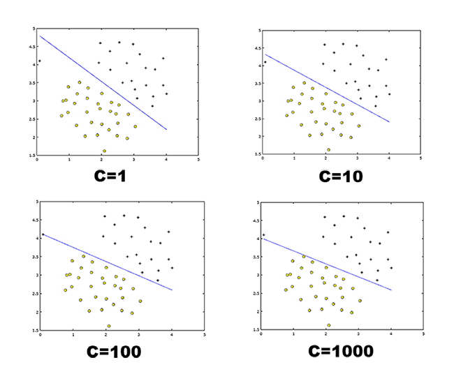
Suppose we have a simple dataset, which is linearly separable like in Figure 1
Figure 1: Linear separable dataset
We use different values of the parameters to illustrate how the decision boundaries varies in each when = 1,10,100 and 1000 in Figure 2.
 Figure 2: Linear decision boundaries produced using different values.
Notice how affects the decision boundary. A large tells the SVM to try to classify all the examples correctly, which do not really maximize the margin between the two classes (positive and negative) and results in over-fitting. If we have outlier examples that we do not want to affect the decision boundary, then we can reduce . plays a role similar to , where is the regularization parameter that we we using previously for logistic regression.
Gaussian Kernel
Now to the more interesting part, we will use SVM to do non-linear classification with the Gaussian kernels. Kernels enable us to make complex and non-linear classifiers using SVM. The idea behind this concept is that, given , we compute new feature depending on proximity to landmarks , , …
To achieve this this, we will first need to find the “similarity” of and some landmark , i.e.
% matlab implementation
sim = exp(-sumsq(x1-x2)/(2*(sigma^2)));
This “similarity” function is what we refer as Gaussian Kernel. There are a few interesting properties of Gaussian Kernel:
- When , then
- When is far from , then
Each of the landmark gives us the features in our hypothesis
is a parameter of the Gaussian Kernel, and it can be modified to increase or decrease the drop-off of our feature , which brings us to the next question, where and how do you produce landmarks?
One way to get the landmarks is to put them in the exact same locations as all the training examples, resulting in landmarks, with one landmark per training example, i.e.
, ,
With this, we can use the SVM minimization algorithm but with substituted in for :
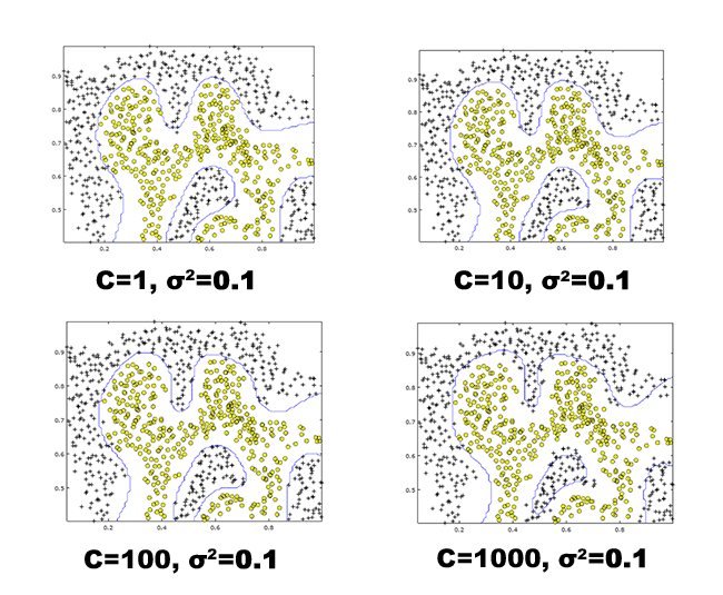
For a non-linear problem, like in Figure 3, we will use SVM with Gaussian Kernel with different settings to understand how decision boundaries will differ.
Figure 3: Non-linear separable dataset
Again, to illustrate how the effects of affects the decision boundary, we will use
We use different values of the parameters to illustrate how the decision boundaries varies in each when = 1,10,100 and 1000 with fixed at 0.01 in Figure 4.
 Figure 4: Non-linear decision boundaries produced using different values with fixed at
 0.01.
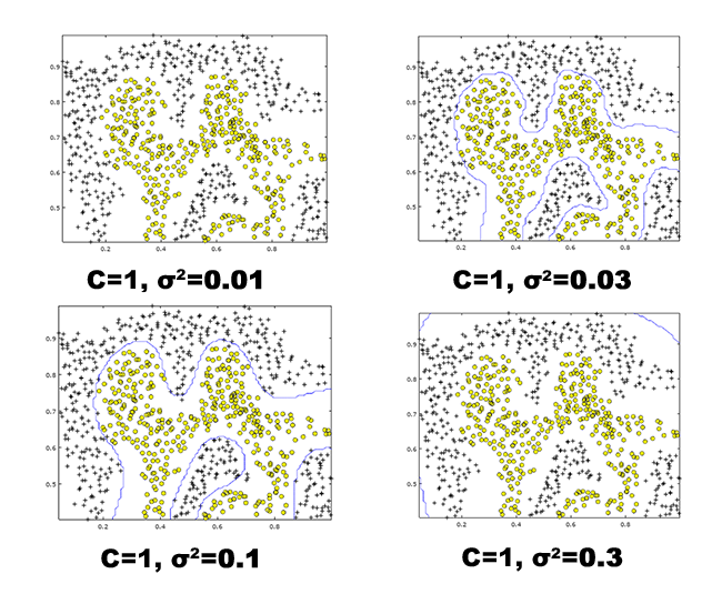
Since it is obvious that when = 1 gives us the best boundary among the other tested values, we will fix this value and change the value. This will help us understand the effects of it towards the decision boundaries. We will test with values = 0.01, 0.03, 0.1 and 0.3.
 Figure 5: Non-linear decision boundaries produced using different values with fixed at
 1.
Comparing this two different parameter between and , it is obvious that has a greater ‘disruptive’ effects towards the decision boundary, where a slight change of it will very much change the entire landscape of the decision boundary.
Email Spam Classifier
Next, we will build our spam classifier using SVM to filter emails (linearly separable dataset in this case). We will only be using the body of the email (excluding headers). Suppose we have the following chunk of text below
Anyone knows how much it costs to host a web portal ?
Well, it depends on how many visitors you’re expecting. This can be anywhere from less than 10 bucks a month to a couple of $100. You should checkout http://www.rackspace.com/ or perhaps Amazon EC2 if youre running something big..
To unsubscribe yourself from this mailing list, send an email to: groupname-unsubscribe@egroups.com
Before building our SVM classifier, it is important to pre-process our data, especially when we are dealing with text. This will essentially improves the performance. Typical text preprocessing includes:
- Lower-casing: The entire email is converted into lower case
- Stripping HTML: Removing HTML tags, so can we retain only the contents
- Normalizing URLs: All URLs are replace with the text “httpaddr”
- Normalizing Email Addresses: All email addresses are replaced with the text “emailaddr”
- Normalizing Numbers: All numbers are substituted with “number”
- Word Stemming: Words are reduced to their stemmed form
- Removal of non-words: Non-words and punctuation have been removed.
% Preprocessing text using Regular Expressions
% Lower case
email_contents = lower(email_contents);

% Strip all HTML
% Looks for any expression that starts with < and ends with > and replace
% and does not have any < or > in the tag it with a space
email_contents = regexprep(email_contents, '<[^<>]+>', ' ');

% Handle Numbers
% Look for one or more characters between 0-9
email_contents = regexprep(email_contents, '[0-9]+', 'number');

% Handle URLS
% Look for strings starting with http:// or https://
email_contents = regexprep(email_contents, ...
                           '(http|https)://[^\s]*', 'httpaddr');

% Handle Email Addresses
% Look for strings with @ in the middle
email_contents = regexprep(email_contents, '[^\s]+@[^\s]+', 'emailaddr');
After preprocessing, our original chunk of text will look like
==== Processed Email ====
anyon know how much it cost to host a web portal well it depend on how mani visitor you re expect thi can be anywher from less than number buck a month to a coupl of dollarnumb you should checkout httpaddr or perhap amazon ecnumb if your run someth big to unsubscrib yourself from thi mail list send an email to emailaddr
After cleaning, we will extract the feature that converts each email into a vector. Where we will count the occurrence of a particular word in an email. Then, we will load it into our SVM classifier. Once the training completes with = 1, we will be expecting a training accuracy of approximately 99.9% and a test accuracy of about 97.7%.
To understand what makes an email to be classified as spam, we can take a look at the top predictors of spam:
our             (0.720293)
flash           (0.561777)
wi              (0.557910)
numberb         (0.550848)
remov           (0.533084)
visit           (0.488539)
click           (0.486210)
bodi            (0.469367)
guarante        (0.460334)
tel             (0.457512)
instruct        (0.455643)
send            (0.453376)
basenumb        (0.412961)
tm              (0.408305)
dollarnumb      (0.408257)
Using the previous chunk of text, our classifier to predict as spam.
Spam Classification: 1
1 indicates spam, 0 indicates not spam)
Using another text example:
Folks,
my first time posting - have a bit of Unix experience, but am new to Linux.
Just got a new PC at home - Dell box with Windows XP. Added a second hard disk for Linux. Partitioned the disk and have installed Suse 7.2 from CD, which went fine except it didn’t pick up my monitor.
I have a Dell branded E151FPp 15” LCD flat panel monitor and a nVidia GeForce4 Ti4200 video card, both of which are probably too new to feature in Suse’s default set. I downloaded a driver from the nVidia website and installed it using RPM. Then I ran Sax2 (as was recommended in some postings I found on the net), but it still doesn’t feature my video card in the available list. What next?
Another problem. I have a Dell branded keyboard and if I hit Caps-Lock twice, the whole machine crashes (in Linux, not Windows) - even the on/off switch is inactive, leaving me to reach for the power cable instead.
If anyone can help me in any way with these probs., I’d be really grateful - I’ve searched the ‘net but have run out of ideas.
Or should I be going for a different version of Linux such as RedHat? Opinions welcome.
Thanks a lot, Peter
– Irish Linux Users’ Group: ilug@linux.ie http://www.linux.ie/mailman/listinfo/ilug for (un)subscription information. List maintainer: listmaster@linux.ie
Spam Classification: 0
1 indicates spam, 0 indicates not spam)
Again, notice the difference between these two chunk of text, while the former chunk of text may look the typical email that went to our spam folder, and the latter may look more like a legit email.
Conclusion
By now, we learned that SVM is actually a modification of logistic regression, so when do we use SVM and when do we use logistic regression?
-
Case 1: If our number of features, , is large (relative to our number of examples ), then we use logistic regression, or SVM without a kernel, since we do not have enough examples to need a complicated polynomial hypothesis.
-
Case 2: If is small and is intermediate, then use SVM with a Gaussian Kernel, since we have enough examples that we may need a complex non-linear hypothesis.
-
Case 3: If is small and is large, then we manually add/create more features, then use logistic regression or SVM without a kernel, since we want to increase our features so that logistic regression becomes applicable.
To summarize, the table below provides the strengths and weaknesses of SVM
| Strengths | Weaknesses |
|---|---|
| Can be used for classification or numeric prediction problems | Finding the best model requires testing of various combinations of kernels and model parameters |
| Not overly influenced by noisy data and not very prone to over-fitting | Can be slow to train, particularly if the input dataset has a large number of features or examples |
| May be easier to use than neural networks, particularly due to the existence of several well-supported SVM algorithms | Results in a complex black box model that is difficult, if not impossible, to interpret |
| Gaining popularity due to its high accuracy and high-profile wins in data mining competitions |