Regularized Linear Regression vs Regularized Polynomial Regression and Bias-Variance Trade-off

Hello everyone, Happy 2018 and welcome back!

Up until now, we have discussed a few interesting machine learning algorithms that is capable of solving complex problems. Although it is important to understand the underlying mathematical theory of each algorithm, we should also begin to question, how can we further improve our algorithm? If we discover that our algorithm is under-performing (i.e. the margin of errors are big), what should we do?

According to Andrew, errors in our predictions can be troubleshooted by:

Getting more training examples
Trying smaller sets of features
Trying additional features
Trying polynomial features
Increasing or decreasing $\lambda$

We will delve into diagnostic techniques for choosing one of the above solutions in this post! We will implement regularized linear regression to predict the amount of water flowing out of a dam using the change of water level in a reservoir, then we will apply it to examine models with different bias-variance properties.

In previous post, we have discussed pretty much on how well our algorithm are trained. This gave us a good idea on how it worked on the training set, but we have no idea on how well the algorithm is performing in our test set. To work it out, we will first divide our dataset into three different parts, with 60% of training set, 20% of cross validation set, and 20% of test set:

Training set (where our model learn on X, y) - 60%
Cross validation set (where regularization parameter Xval and yval are determined) - 20%
Test set (where the performance is evaluated. These are unseen examples which our model did not see during training: Xtest, ytest) - 20%

However, splitting based on this percentage is subjective and might varies according to situation. There are few good discussions on how should we split our dataset on CrossValidated that is worth reading for more comprehensive understanding towards this subject.

Back to our Regularized Linear Regression problem, we will first visualize our data by plotting it out.

% Plot training data
plot(X, y, 'rx', 'MarkerSize', 10, 'LineWidth', 1.5);
xlabel('Change in water level (x)');
ylabel('Water flowing out of the dam (y)');

Figure 1: Visualizing the data

Recall that regularized linear regression has the following cost function

$J(\theta)=\frac{1}{2m} \left( \sum_{i=1}^m (h_\theta(x^{(i)})-y^{(i)})^2 \right) + \frac{\lambda}{2m} \left( \sum_{j=1}^n \theta_j^2 \right)$

Correspondingly, the partial derivative of regularized linear regression’s cost for $\theta_j$ is defined as

$\frac{\delta J(\theta)}{\delta\theta_j}=\frac{1}{m}\sum_{i=1}^m(h_\theta(x^{(i)})-y^{(i)})x_j^{(i)} \qquad for \quad j=0$ $\frac{\delta J(\theta)}{\delta\theta_j}=\left( \frac{1}{m}\sum_{i=1}^m(h_\theta(x^{(i)})-y^{(i)})x_j^{(i)} \right) + \frac{\lambda}{m}\theta_j \qquad for \quad j \geq 1$

where $\lambda$ refers to the regularization parameter which governs the degree of regularization. This regularization term puts a penalty on the overall cost value $J$ , that is, when the magnitudes of the model parameters $\theta_j$ increases, the penalty increases too. When $\theta$ is initialized to theta=[1;1], we expect our cost value to be approximately at 303.99.

%MATLAB/OCTAVE Implementation
% fraction of linearRegCostFunction function

%cost function
J = (1/(2*m))*sum(power((X*theta - y),2))+ (lambda/(2*m)) * sum(power(theta(2:end),2));

% for j >=1
regularized = (lambda/m) .* theta;
% for j = 0
regularized(1) = 0;

grad = ((1/m) .* X' * (X*theta - y)) + regularized; 

Cost at theta = [1 ; 1]: 303.993192

Since the dataset is of such low dimension , where we are trying to fit a 2D $\theta$ , regularization will not be playing a crucial part, we will set our regularization parameter $\lambda$ = 0 for this part. Furthermore, when plotting the best fit line to our data in Figure 2, we notice that it is not a good fit to the data since the data is non-linear in nature. To fit this dataset better, we will use polynomial regression in later part. We will first implement a function to generate learning curves that can help us debug our learning algorithm.

Figure 2: Linear fit is not a a good fit to our data

Bias-Variance Trade-off

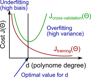
Before that, an useful concept in machine learning to bring out is the bias-variance trade-off. In simple words, a high-bias model is not complex enough for the data and might result to under-fitting. On the contrary, a high-variance model is too complex for the data and might result to over-fitting. If you are puzzled, just remember the acronym - BUVO (Bias, Under-fit; Variance, Over-fit) !

Learning Curves

Learning curves basically plots training and cross validation error as a function of training set size and it is a useful method in debugging learning algorithms, where the error function for our training set is defined as

$J_{train}(\theta) = \frac{1}{2m} \left[ \sum_{i=1}^m (h_\theta(x^{(i)}-y^{(i)})^2 \right]$

Similarly, our error function for our cross validation set is defined as

$J_{CV}(\theta) = \frac{1}{2m} \left[ \sum_{i=1}^m (h_\theta(x^{(i)}-y^{(i)})^2 \right]$

for i = 1:m
  % splitting training dataset
  X_train = X(1:i, :);
  y_train = y(1:i, :);
  
  theta = trainLinearReg(X_train, y_train, lambda);
  
  error_train(i) = linearRegCostFunction(X_train, y_train, theta, 0);
  error_val(i) = linearRegCostFunction(Xval, yval, theta, 0);

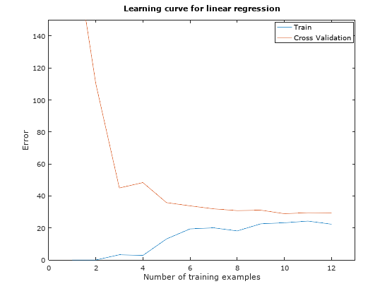
Once implemented, the error of the training set and cross validation set will be computed and the learning can be plotted out and will look like in Figure 3.

% Computing the first train error of training set and cross validation set for linear regression
# Training Examples     Train Error     Cross Validation Error
            		0.000000        205.121096
            		0.000000        110.300366
            		3.286595        45.010231
            		2.842678        48.368911
           		13.154049       35.865165
            		19.443963       33.829962
            		20.098522       31.970986
            		18.172859       30.862446
            		22.609405       31.135998
           		23.261462       28.936207
            	24.317250       29.551432
            	22.373906       29.433818

Figure 3: Linear regression learning curve

Notice that as the number of training examples increase, both training set error and cross validation error remained at a high error value. This indicates a high bias problem in our model, where the linear regression model is under-fitting and is unable to fit our dataset very well. To obtain a better fit to our model, we will introduce polynomial regression.

Polynomial Regression

In simple words, polynomial regression add more features to our hypothesis such that

$h_\theta(x)=\theta_0+\theta_1*(x_1)+\theta_2*(x_2)^2+ ...+ \theta_p*(x_p)^P$

where $x$ is the feature of your dataset. Let’s say we want to map our hypothesis to the $p^{th}$ polynomial, we can do this by

for i = 1:p
  X_poly(:,i) = X.^i;  
end

In this post, we will use a polynomial degree of 8 for the sake of discussion, where feature normalization is applied to scale our dataset better. Once the parameters $\theta$ are learnt using $\lambda$ =0, we can compute the training set and cross validation set error and plot the polynomial fit and the learning curve as depicted in Figure 4 and Figure 5.

% Computing the first train error of training set and cross validation set for polynomial regression
# Training Examples     Train Error     Cross Validation Error
            		0.000000	160.721900
            		0.000000	160.121510
            		0.000000	61.754825
            		0.000000	61.928895
           		0.000000	6.597913
            		0.000191	10.239934
            		0.040538	8.039769
            		0.076369	5.293786
            		0.162867	7.196048
           		0.150745	8.828604
            	0.162416	10.133383
            	0.084463	7.734434

Figure 4: Polynomial fit when $\lambda$ = 0

Figure 5: Polynomial learning curve when $\lambda$ = 0

Comparing these set of output relative to the ones we obtained using linear regression model, we observe a better fitting of the model to the dataset and the learning curve is able to records very little errors as the number of training data increases. However this is another typical example of over-fitting. Hence, we will need to consider regularization in this case, where we will tune the polynomial fitting and learning curve using different value for $\lambda$ , where $\lambda$ = 0.1, 1, 3,10 and 100 respectively. Figure 6 compares the result of each $\lambda$ value.

Figure 6: Polynomial fittings and learning curves when $\lambda$ = [0.1,1,3,10,100]

It is obvious that the value of $\lambda$ can significantly affect the results of regularized polynomial regression on the training set and cross validation set. A model without regularization or small regularization fits the training set well, but does not generalize well, causing over-fitting. On the contrary, a model with too much regularization does not fits the training set well, causing under-fitting. A better choice of $\lambda$ will the ones when $\lambda$ = 1 or 3.

Conclusion

As discussed here, plotting the learning curves to understand what problem (whether a bias or variance problem) our current dataset is experiencing is a crucial procedure to understand how well our machine learning algorithm is working. To recap, remember

High Bias = Under-fitting (BU): both $J_{train}(\theta)$ and $J_{CV}(\theta)$ will be high. Also, $J_{train}(\theta) \approx J_{train}(\theta)$

High Variance = Over-fitting (VO): $J_{train}(\theta)$ will be low and $J_{CV}(\theta)$ will be much greater than $J_{train}(\theta)$

Figure 7: BU-VO!

To conclude, the following table summarizes the different approaches one way consider when debugging a learning algorithm.

	Fixes Problem of
Get more training examples	High Variance
Try smaller sets of features	High Variance
Try getting additional features	High Bias
Try adding polynomial features	High Bias
Try decreasing $\lambda$	High Bias
Try increasing $\lambda$	High Variance

References

1. Ng, A. “Machine Learning” [Week 6 Lecture Notes]. MOOC offered by Stanford University, Coursera. Retrieved on January 7, 2018 from https://www.coursera.org/learn/machine-learning/resources/LIZza