Handwriting recognition using Artificial Neural Network

An Artificial Neural Network (ANN) or generally known as Neural Network models the relationship between a set of input signal (dendrites)and on output signal (axons) using a model derived from our understanding of how a biological brain responds to stimuli from sensory inputs. Let us examine how we will represent a hypothesis function using Neural Network!

In our model, our dendrites are like the input features $x_1,...x_n$ and the output is the result of our hypothesis function. Our $x_0$ input node is sometimes called the ‘bias unit’ and always equal to $1$ . We use the same logistic function as in previous classification problems, i.e. $\frac{1}{1+e^{\theta^Tx}}$ . This is usually referred as a sigmoid activation function. Our $\theta$ are sometimes referred as ‘weights’. Visually, a simplistic representation looks like

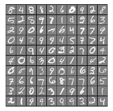
$\begin{bmatrix} x_0 \\ x_1 \\ x_2 \\ \end{bmatrix} \to [\quad] \to h_\theta(x)$

The question is, why Neural Network? Neural Network offers an alternate way to perform machine learning when we have complex hypotheses with many features. In this multi-class classifier problem to recognize handwritten digits, Neural Network is a better choice than logistic regression because logistic regression cannot form more complex hypotheses as it is only a linear classifier. Our dataset contains 5000 training examples of handwritten digits, where each training examples is a 20 x 20 pixel gray scale image of the digit. Each pixel is represented by a floating point number indicating the gray scale intensity at that location. The 20 x 20 grid of pixels in ‘unrolled’ into a 400-dimensional vector. Each of these training examples becomes a single row in our data matrix X, resulting to a 5000 x 400 matrix X where every row is a training example for a handwritten digit image. The second part of the training set is a 5000-dimensional vector y that contains labels for the training set. We have mapped the digit zero to the value ten. Therefore, a 0 digit is labeled as 10, white the digits 1 to 9 are labeled as 1 to 9 in their natural order.

Figure 1: Random 100 rows from our dataset

Model Representation

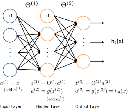
We will implement a feed-forward propagation neural network algorithm in order to use our weights for prediction. Figure 1 shows a more detailed neural network representation.

Figure 2: Neural Network model

Our input nodes (layer 1) go into another node (layer 2), and are output as the hypothesis function. The first layer is called the “input layer” and the final layer the “output layer,” which gives the final value computed on the hypothesis. We can have intermediate layers of nodes between the input and output layers called the “hidden layer.” We label these intermediate or “hidden” layer nodes $a_0^2,...a_n^2$ and call them “activation units”.

For instance, if we had one hidden layer, it would look visually something like

$\begin{bmatrix} x_0 \\ x_1 \\ x_2 \\ x_3 \\ \end{bmatrix} \to \begin{bmatrix} a_1^{(2)} \\ a_2^{(2)} \\ a_3^{(2)} \\ \end{bmatrix} \to h_\theta(x)$

The values for each of the ‘activation’ nodes is obtained as follows:

$a_1^{(2)}=g(\theta_{10}^{(1)}x_0+\theta_{11}^{(1)}x_2+\theta_{12}^{(1)}x_2+\theta_{13}^{(1)}x_3) \\ a_2^{(2)}=g(\theta_{20}^{(1)}x_0+\theta_{21}^{(1)}x_2+\theta_{22}^{(1)}x_2+\theta_{23}^{(1)}x_3) \\ a_3^{(2)}=g(\theta_{30}^{(1)}x_0+\theta_{31}^{(1)}x_2+\theta_{32}^{(1)}x_2+\theta_{33}^{(1)}x_3) \\ h_\theta(x)=a_1^{(3)}=g(\theta_{10}^{(2)}a_0^{(2)}+\theta_{11}^{(2)}a_1^{(2)}+\theta_{12}^{(2)}a_2^{(2)}+\theta_{13}^{(2)}a_3^{(2)})$

Although it may seem complex theoretically, but using a powerful concept called vectorization, we only requires few lines of code in MATLAB/OCTAVE to fully implement this idea. Pretty DOPE!

% adding one more columns (bias value) of 1's to the first layer
a1 = [ones(m,1) X];
% compute activation units
a2 = sigmoid(a1 * Theta1');
% again, adding one more column (bias value) to the exisiting a2
a2 = [ones(size(a2,1),1) a2];
% compute activation units
a3 = sigmoid(a2 * Theta2');
% same in multi-class classification, we want to get the max_value
% and also the index of it
[max_value, p] = max(a3, [], 2);

Multi-class Classification

Since we want to classify data into multiple classes, we let our hypotheses function return a vector of values. Say we wanted to classify our data into one of four final resulting classes:

$\begin{align*}\begin{bmatrix}x_0 \newline x_1 \newline x_2 \newline\cdots \newline x_n\end{bmatrix} \rightarrow\begin{bmatrix}a_0^{(2)} \newline a_1^{(2)} \newline a_2^{(2)} \newline\cdots\end{bmatrix} \rightarrow\begin{bmatrix}a_0^{(3)} \newline a_1^{(3)} \newline a_2^{(3)} \newline\cdots\end{bmatrix} \rightarrow \cdots \rightarrow\begin{bmatrix}h_\theta(x)_1 \newline h_\theta(x)_2 \newline h_\theta(x)_3 \newline h_\theta(x)_4 \newline\end{bmatrix} \rightarrow\end{align*}$

Our final layer of nodes, when multiplied by its theta matrix, will result in another vector, on which we will apply the $g()$ logistic function to get a vector of hypothesis values, which look like:

$h_\theta(x) =\begin{bmatrix}0 \newline 0 \newline 1 \newline 0 \newline\end{bmatrix}$

In which case our resulting class is the third one down, or $h_\theta(x)_3$ . We can define our set of resulting classes as y, where

$y^{(i)}=\begin{bmatrix}1\\0\\0\\0 \end{bmatrix}, \begin{bmatrix}0\\1\\0\\0 \end{bmatrix}, \begin{bmatrix}0\\0\\1\\0 \end{bmatrix}, \begin{bmatrix}0\\0\\0\\1 \end{bmatrix}$

Our final value of our hypothesis for a set of inputs will be one of the elements in y.

Results

Time to test how well did our model performs. We will try to input a digit in gray scale format and see what does the neural network predicts

Figure 3: Digit 6 in gray scale

Neural Network Prediction: 6 (digit 6)

Figure 4: Digit 6 in gray scale

Neural Network Prediction: 6 (digit 6)

Figure 5: Digit 4 in gray scale

Neural Network Prediction: 4 (digit 4)

Figure 6: Digit 8 in gray scale

Neural Network Prediction: 8 (digit 8)

Figure 7: Digit 9 in gray scale

Neural Network Prediction: 9 (digit 9)

Took me quite a while (after 48 consecutive correct predicts) to finally encounter with a wrong prediction! The Neural Network some how get ‘confused’ between digit 6 and digit 9.

Figure 8: Digit 9 in gray scale

Neural Network Prediction: 6 (digit 6)

Our multi-class Neural Network was capable to record a decent accuracy of 97.5.

Training Set Accuracy: 97.520000

This is just the very tip of the iceberg for this amazing yet complex algorithm. We will discuss in more detail and an important part of Neural Network which covers back-propagation in the upcoming post. Stay tuned, and bye for now!

References

1. Ng, A. “Machine Learning” [Programming Exercise 3: Multi-class Classification and Neural Network]. MOOC offered by Stanford University, Coursera. Retrieved on December 23, 2017 from https://www.coursera.org/learn/machine-learning/resources/JOjNO