Microchip QA Test Classifier with Regularized Logistic Regression

From our previous post, we understand that most real-world problems are not linearly separable, which means our dataset cannot be separated into positive and negative examples by a straight-line through a plot. Now, let us take a look on how this issue of be addressed.

We will implement a regularized logistic regression to predict whether microchips from a fabrication plant passes quality assurance (QA) using historical data. During QA, each microchip goes through various tests to ensure it is functioning correctly. Based on our historical data, let us build our logistic regression model.

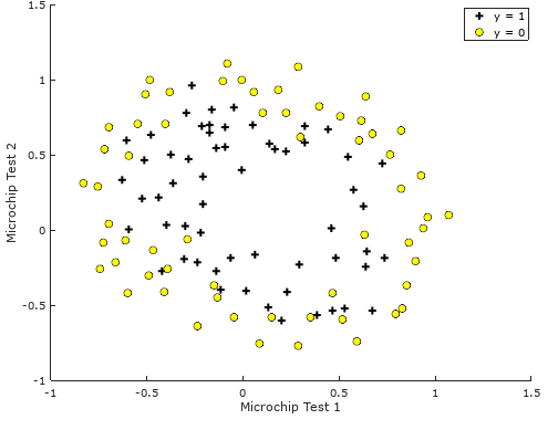
Back to the previously mentioned non-linearly separable problem. Figure 1 shows an example of a problem of such

Figure 1: Visualizing the scatter plot

Since we know that a straight-forward application of logistic regression will not perform well on this dataset, we need to create more features from each data point where we will map the features into all polynomial terms of $x_1$ and $x_2$ up to the sixth power

$mapFeature(x)=1,x_1,x_2,x_1^2,x_1x_2,...,x_1x_2^5, x_2^6$

As a result of this mapping, we will be able to transform our vector into a 28-dimensional vector. A logistic regression classifier trained on this high-dimension feature vector will have a more complex decision boundary and will appear non-linear when drawn in our 2-dimensional plot. While the feature mapping allows us to build a more comprehensive classifier, it is also more susceptible to over-fitting (opposite of under-fitting). Let us compare the difference between them.

Over-fitting	Under-fitting
Also known as High Variance	Also known as High Bias
Caused by a hypothesis function $h$ that fits the available data but does not generalize well to predict new data	Happens when the form of our hypothesis function $h$ maps poorly to the trend of the data.
Usually caused by a complicated function that creates a lot of unnecessary curves and angles unrelated to the data.	Usually caused by a function that is too simple or uses too few features. eg. if we take $h_\theta(x)=\theta_0+\theta_1x_1+\theta_0x_2$ , then we are making an initial assumption that a linear model will fit, the training data well and will be able to generalize but that may not be the case.

One way to overcome over-fitting is through regularization, where what is actually done is just merely reducing the parameters $\theta_j$ while keeping all the features. To achieve this idea, we introduce our regularization parameter, $\lambda$ . The regularized cost function in logistic regression is as follows

$J(\theta)=\frac{1}{m}\sum_{i=1}^m [-y^{(i)}\log(h_\theta(x^{(i)}))-(1-y^{(i)})\log(1-h_\theta(x^{(i)}))]+\frac{\lambda}{2m}\sum_{j=1}^n\theta_j^2$

The gradient of the cost function is a vector where the $j^{th}$ element is defined as follows (note that we should not regularize the parameter $\theta_j$ )

$\frac{\delta J(\theta)}{\delta\theta_j}=\frac{1}{m}\sum_{i=1}^m(h_\theta(x^{(i)})-y^{(i)})x_j^{(i)}\qquad (for\quad j=0)$ $\frac{\delta J(\theta)}{\delta\theta_j}=\Biggl(\frac{1}{m}\sum_{i=1}^m(h_\theta(x^{(i)})-y^{(i)})x_j^{(i)})\Biggr)+\frac{\lambda}{m}\theta_j\qquad (for\quad j\ge 1)$

Once this is implemented, we computed our cost function using the initial value of $\theta$ (initialized to all zeros), we are able to get the cost around 0.693. If we were to change $\lambda=10$ , we would expect our cost to be 3.165.

Cost at initial theta (zeros): 0.693147
Cost at test theta (with lambda = 10): 3.164509

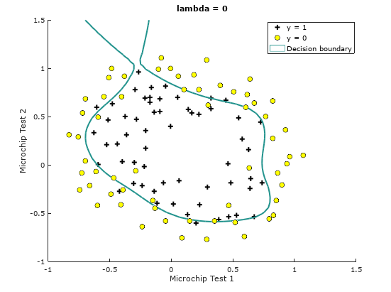
Let us visualize how does the decision boundary behaves with $\lambda=0$ . Figure 2 shows the decision boundary based on this setting.

% we will try lambda = 1, 10 and 100 too later
lambda = 0;

% Set Options
options = optimset('GradObj', 'on', 'MaxIter', 400);
% Optimize
[theta, J, exit_flag] = fminunc(@(t)(costFunctionReg(t, X, y, lambda)), initial_theta, options);
% Plot Boundary
plotDecisionBoundary(theta, X, y);
% Compute accuracy on our training set
p = predict(theta, X);
acc = mean(double(p == y)) * 100);

Figure 2: Training data with decision boundary $\lambda=0$

Train Accuracy (lambda = 0): 86.440678

To better understand the effects of $\lambda$ , precisely on the matter of how regularization prevents over-fitting, let us visualize how the decision boundary behaves and the prediction accuracy varies when using different values of $\lambda$ .

When $\lambda=1$

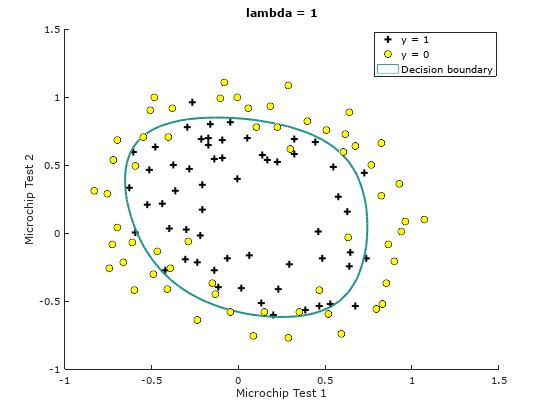
Figure 3: Training data with decision boundary $\lambda=1$

Train Accuracy (lambda = 1): 83.050847

When $\lambda=10$

Figure 4: Training data with decision boundary $\lambda=10$

Train Accuracy (lambda = 10): 74.576271

When $\lambda=100$

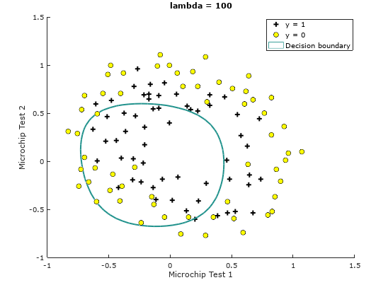
Figure 5: Training data with decision boundary $\lambda=100$

Train Accuracy (lambda = 100): 61.016949

Notice the changes in the decision boundary as we vary $\lambda$ . With a small $\lambda=0$ , we should find that the classifier gets almost every training example correct, but draws a very complicated boundary, thus over-fitting the data like in Figure 2, therefore not a good decision boundary. With a larger $\lambda$ ( $\lambda$ = 1 or $\lambda$ = 10), we should see a plot that shows a simpler and straight-forward decision boundary which still separates the positives and negatives fairly well. However, if $\lambda$ is set to too high ( $\lambda$ = 100), we will not get a good fit and the decision boundary will not follow the data so well, thus under-fitting the data like in Figure 5.

References

1. Ng, A. “Machine Learning” [Programming Exercise 2: Logistic Regression]. MOOC offered by Stanford University, Coursera. Retrieved on December 16, 2017 from https://www.coursera.org/learn/machine-learning/resources/fz4AU