Predicting Student Admission using Logistic Regression
Logistic Regression is another kind of supervised machine learning which is used to model a binary categorical outcome, that is, instead of our output vector being a continuous range of values, it will only be or . Where is usually taken as the negative class and as the positive class, but we are free to assign any representation it.
We will build a logistic regression model to predict whether a student gets admitted into a university based on their examinations result. Suppose we have historical data from previous applicants that we can use as a training set for logistic regression, for each training example, we have the applicant’s scores on two exams and the admissions decision, either or .
A good practice before implementing any learning algorithm is to always visualize the data, if possible.
% Find Indices of Positive and Negative Examples
pos = find(y==1); neg = find(y == 0);
% Plot Examples
plot(X(pos, 1), X(pos, 2), 'k+','LineWidth', 2, 'MarkerSize', 7);
plot(X(neg, 1), X(neg, 2), 'ko', 'MarkerFaceColor', 'y', 'MarkerSize', 7);
Figure 1: Visualizing the scatter plot
Now we have visualized the data, let us dig deeper into mathematical background of logistic regression. The logistic regression hypothesis is defined as:
where function is the sigmoid function. The sigmoid function is defined as:
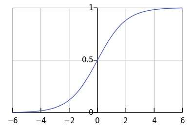
As usual, let us visualize the sigmoid function a.k.a logistic curve using the graph as shown in Figure 2. For large positive values of , the sigmoid should be close to , while for large negative values, the sigmoid should be close to .
 Figure 2: The logistic curve
The cost function for logistic regression that we will be minimizing is
and the gradient of the cost is a vector of the same length as where the element is defined as follows:
Although this gradient looks very similar to the linear regression gradient, do keep in mind that the formula is actually different because linear and logistic regression have different hypotheses . Now that we have all fundamental blocks of information, it is now time to assemble them together! Using initial =0, we obtain
Cost at initial theta (zeros): 0.693147
Gradient at initial theta (zeros):
-0.100000
-12.009217
-11.262842
To minimize it, we apply gradient descent in hope that the solution to converge to a more optimal solution, below is the result
Cost at test theta: 0.218330
Theta:
0.042903
2.566234
2.646797
We will now optimize the cost function with parameters using the built-in function, fminunc, in MATLAB/Octave which aims to find the minimum of an unconstrained function.
% Set options for fminunc
options = optimset('GradObj', 'on', 'MaxIter', 400);
% Run fminunc to obtain the optimal theta
% This function will return theta and the cost
[theta, cost] = ...
fminunc(@(t)(costFunction(t, X, y)), initial theta, options);
After using fminunc, we obtain
Cost at test theta: 0.203498
Theta:
-25.161272
0.206233
0.201470
It is clear that with fminunc, we are able to get a better solution of 0.203498 among the tested approaches. With these settings, let us take a look how does the decision boundary separate our classifier
Figure 3: The decision boundary after training our dataset
Therefore, using our trained model, we can now predict whether a student with get their admission based on their exams result.
Case 1: Student ‘A’ with exams result of 45 and 85.
prob = sigmoid([1 45 85] * theta);
For a student with scores 45 and 85, we predict an admission probability of 0.776289
Case 2: Student ‘B’ with exams result of 35 and 65.
prob = sigmoid([1 35 65] * theta);
For a student with scores 35 and 65, we predict an admission probability of 0.007786
Case 3: Student ‘A’ with exams result of 15 and 35.
prob = sigmoid([1 15 35] * theta);
For a student with scores 15 and 35, we predict an admission probability of 0.00000
From our observation of a size 100, we can then compute the accuracy of our model using
% Compute accuracy on our training set
p = predict(theta, X);
acc = mean(double(p == y)) * 100);
Train Accuracy: 89.000000
This wrap-ups the idea of Logistic Regression, where we can use it model binary categorical outcome. Of course, this post highlight the very surface of this supervised machine learning method, in real-world problems, most of the time the data are not linearly separable. How do we use Logistic Regression to solve problems of such? Stay tunned for the following update!